What are Transformers - Understanding the Architecture End-to-End
Table of Contents
Alejandro Armas and Sachin Loechler have been hard at work on a project that involves developing streaming workloads.
The project has the goal to process realtime data and support real-time traffic prediction! In order to make sense of the enormous quanity of unstructured video data, we employed Foundational models that perform video tracking, bounding box, depth estimation and segmentation to extract information from video data. Many of these foundational models relied on an artificial Neural Network Architecture called a Transformer. I want to add my perspective on how all these pieces fit together so I hope you enjoy.
💡 BIG IDEA: The Self-Attention module is used in three different places. It is a subtle difference between each of the three
I’ll explain the difference between where the self-attention modules find themselves. For now, understanding some of the bigger concepts will help in that.
For this blogpost, I’ll be using text data to help you understand the concepts behind a Transformer Architecture better. Just because LLMs blew up in popularity, there is no requirement for a transformer to require text data. In general, one could use any form of sequential or ordered data.
Data Source
So, we could have a single sentence "Hello World, this is Alejandro!" and want to create a dataset to the tune of:
We have a special token signifying the beginning of the sequence and another signifying the end of the sequence.
Tokenize Text
We develop a strategy to tokenize our text. This means converting our raw string of text into a sequence of integers according to some vocabulary.
In our example, we are going to convert individual words into integers. First we begin by appending a special character to both the start and end, then we are able to split the string into a list of words. The set data structure handles duplicates for us.
text = '<SOS> Hello World, this is Alejandro! <EOS>'
words = sorted(list(set(text.split(' '))))
To make things simple, we can iterate over our list and enumerate each word.
stoi = { w:i for i,w in enumerate(words) } # maps tokens to integers
itos = { i:w for i,w in enumerate(words) } # maps integers to tokens
encode = lambda s: [stoi[w] for w in s] # encoder: take a string, output a list of integers
decode = lambda l: ''.join([itos[i] for i in l]) # decoder: take a list of integers, output a string
Great we have just created the functions neccessary to tokenize our text. You can also check out SentencePiece and TikToken for tokenizers used in practice.
print(encode(text.split(' ')))
> ['<EOS>', '<SOS>', 'Alejandro!', 'Hello', 'World,', 'is', 'this']
print(torch.tensor(encode(text.split(' ')), dtype=torch.long))
> data=tensor([1, 3, 4, 6, 5, 2, 0])
Here we can see the independent variable and dependent variable pairs that will constitute our supervised machine learning problem.
> torch.Size([7]) torch.int64
> when input is tensor([1]) the target: 3
> when input is tensor([1, 3]) the target: 4
> when input is tensor([1, 3, 4]) the target: 6
> when input is tensor([1, 3, 4, 6]) the target: 5
> when input is tensor([1, 3, 4, 6, 5]) the target: 2
> when input is tensor([1, 3, 4, 6, 5, 2]) the target: 0
Awesome! Now we have 6 examples, sampled from a probability distribution representing the semantics and ideas of English Language. Imagine if you built a web-crawler, scraped all the text on the internet (about 10TB of data) and used 6000 GPUs for 12 days ( \(1^{24}\) floating point opererations per second) to induce the statistical makeup of human language into your LLMs model weights… that’s a lot of samples!!
One Hot Encoder
Neural Networks process data through linear algebra operations, so one-hot encoding is a common approach for transforming text data into numbers.
One-Hot Encoder:
Lets say we have a vocabulary of 10000 tokens that represents the English language. A Token is a subunit of words. Tokens can be works, characters or symbols depending on the tokenizer.
Lets break up one of the samples from the previous section (i.e. \(X_1\) ) into a bunch of tokens. For simplicity, the tokenizer breaks words into tokens, so we’d expect the one-hot vector \(\vec{O}_{\text{Hello}} \in \mathbb{R}^{10000}\) representing “Hello” to look like the following:
The purpose behind this is to map each token in our vocabulary to a unique numerical representation. We have all zero’s except for one of the dimension’s entry is set to one.
Embedding Layer
Great, we have all of our tokens, represented by one-hot vectors, functionally acting as a basis vector for this vector space. They are all orthogonal to eachother. Which isn’t the best, since some words have closer meanings to other ones. Its also a wasteful representation, due to its sparsity (i.e. lots of zeroes!).
💡 BIG IDEA: Embedding Layer performs a linear transformation to condense one-hot vectors into a more compact and useful representation, that still preserves the important relationships between all the tokens.
Input Embedding: Transformer takes a sequence of tokens as input, however each token is represented as a vector.
Suppose we are using a 512-dimensional embedding, then each token \(\vec{e}_{\text{Hello}} \in \mathbb{R}^{512}\) is obtained by transforming the one-hot vector with an embedding layer.
You can think of the embedding layers as a lookup table, where each row corresponds to a word or input, and each column corresponds to a feature or dimension.
The embeddings are adjusted according to the context and the task of the Transformer. In our example, we should expect similar words to have a smaller angle between eachother (ex. “Cat” and “Lion”) versus different words (ex. “Headphones” and “Rat”)
Architecture Details
Now before we dive deeper into the post, I want to give you an idea of the architectural choices in Attention Is All You Need versus the simplified example my blogpost showcases
- Embedding dimension \(d_{\text{model}} = 512\) : (4 in our example)
- Number of encoders \(N = 6\) :(2 in our example)
- Number of decoders \(N = 6\) : (2 in our example)
- Feed-forward dimension \(d_{\text{ff}} = 2048\) : (8 in our example)
- Number of attention heads \(h = 8\) : (2 in our example)
- Attention dimension \(d_{\text{k}} = 64\) : (4 in our example)
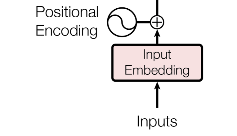
Positional Encoding
💡 BIG IDEA: The Attention Layers within Transformers, unlike RNNs and CNNs don’t have an inherent sense of position or order of data.
RNNs use recurrence and CNNs use the convolution operator to have a sense of position. This is where positional encoding comes into play. Positional Encodings are meant to provide a kind of information (i.e. positional information) that is different from the information provided by word embeddings (i.e. semantic meanings).
Why Positional Encodings
The choice between fixed (like sinusoidal) and learned positional encodings can depend on the specific requirements of your task and data.
You might think the choice of using a sinusoidal function is arbitrary, but it actually provides some useful properties for positional encoding.
- Unique Encodings: Sinusoidal functions, given that they have different frequencies, can generate a unique encoding for the position of each token
- Relative Position Information: For any fixed offset \(\delta\) , a positional encoding \(\vec{p_t}\) can be represented as a linear function of \(\vec{p_{t + \delta}}\)
- Unbounded Domain: Sinusoidal functions are periodic, therefore this provides us with a flexible approach to working with variable input sequences
- Efficient Computation: Sinusoidal functions are easy to compute
We pertubate the input embeddings, that represent the word tokens, by an angle represented by the positional encodings to give each word a small shift in vector space toward the position the word occurs in.
⁉️ How do I know the pertubation imposed by the positional encoding doesn’t coincide with semantic meaning?
The word embedding space captures the semantic meanings learned during the training process, based on the statistical properties of the language data the model is trained on. Therefore, one would not expect that the specific directions in the high-dimensional space that correspond to semantic differences between words would align with the sinusoidal curves used for positional encodings.
Positional Encoding Formula
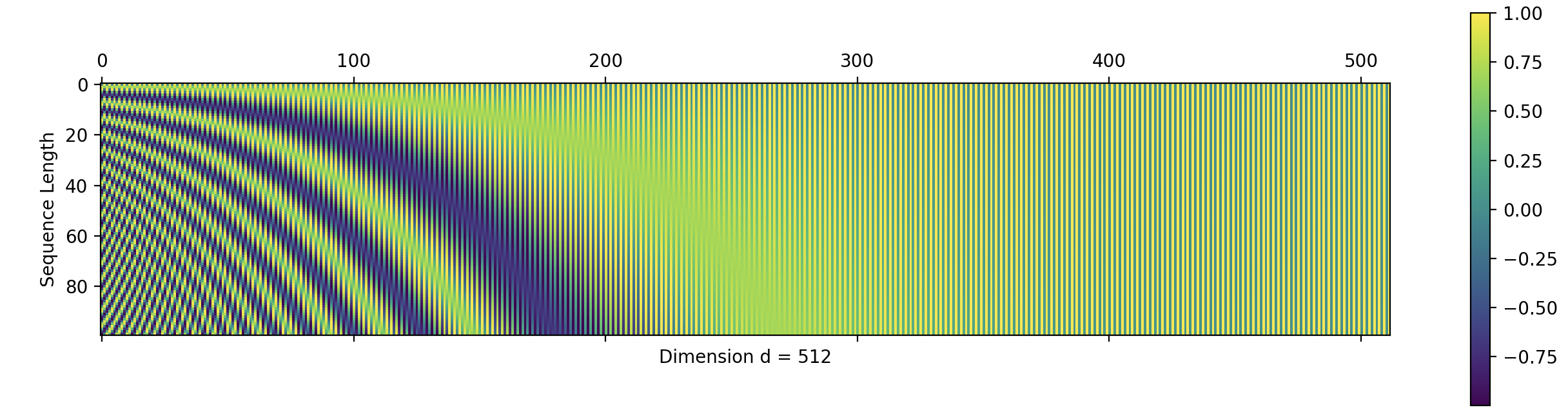
Here we have a 512-dimensional positional encoding. The maximum sequence length of 100 tokens is represented by the number of rows, denoting a single positional encoding \(\vec{p_t}\) .
Let \(t\) be the desired position in an input sentence, \(\vec{p_t} \in \mathbb{R}^d\) be the positional encoding, and \(d\) be the encoding dimension (where \(d \equiv_2 0\) ). That is, \(d\) is an even number. Then, \(PE : \mathbb{N} \to \mathbb{R}^d\) will be the function that produces the corresponding encoding. Here is the formula for the dimension \(i \in \{1, 2, \cdots, d\}\) : Source
Depending on the value of \(i\) , we are able to attain a unique constituent waveform. As \(i\) increases, it changes the period of the waveform to shorter. In other words, the frequency is increased and the function repeats itself more rapidly.
So there you go, depending on the timestep \(t\) , we are able to compute a unique positional encoding.
Positional Encoding Calculation
We are going to calculate the positional encodings of the data sample:
\(X_5\)
= Hello World, this is Alejandro!.
Like I said, we are working with an embedding dimension of four (i.e. \(e_t \in \mathbb{R}^4\) ).
Excluding the start-of-sentence and end-of-sentence tokens, we have 5 unique tokens from this sequence. We’re going to run with this example for awhile, so stick with me. That means the token \(t_0 = \text{'Hello'}\) and the token \(t_3 = \text{'is'}\) .
After representing each token with a one-hot-vector and we might end up with token \(t_3\) corresponding to the following embedding:
Lets calculate the positional encoding for the token "is":
The final embedding after it has been perturbed by the positional encoding is:
I’m not convinced the Positional Encoding is Relative
Lets say that you have a hunch that positonal encoding MIGHT NOT actually offer any relative positional information. That is, you think that for some \(\delta\) it represents a shift that is not dependent on \(\delta\) and instead dependant on the position of the token \(t\) .
Now for positional encoding, we have two cases depending on the value of \(i\) being even or odd.
Case 1: Now, let’s consider two positions, \(t\) and \(t+ \delta\) for some fixed offset \(\delta\) where \(i\) is even. The difference in their positional encodings for a given dimension \(i\) is:
For a fixed \(i\) the difference between the positional encodings is a function of the offset \(\delta\) alone and not the positions themselves \(t\) and \(t + \delta\) .
Case 2: This is very similar to the first case, but instead with an odd \(i\) , so I’ll leave it as an exercise for you.
Encoder
Encoder: Composed of a stack of identical sub-layers. Each sub-layer contains two types of networks:
- multi-head self-attention mechanism
- position-wise fully connected feed-forward network
The output of each sub-layer is normalized using a layer normalization technique.
Self Attention Mechanism
If I’m a noun, maybe I want to look at vowels in the past and place more importance on those versus other words. Also, I would like to do this in a data-dependant way.
import torch # we use PyTorch: https:\\pytorch.org
import torch.nn as nn
from torch.nn import functional as F

B,T,C = 1,5,4 # batch, time, channels
X = torch.randn(B,T,C)
![[Pasted image 20240104130645.png]]
💡 BIG IDEA: Tokens in a sequence interact with all other tokens of the sequence and want to discriminate on where they ought to place their focus. This is done through the learned linear-transformations that map the input tokens into three separate spaces.
💡 BIG IDEA: Since the transformation is performed on the same source, it is considered Self-Attention. In principle, Attention is more generalized.
In the previous section, we derived a final input to the encoder \(\vec{x}_3\) :
print(f'{X[0, 3, :]}')
> tensor([[0.3411, 1.2990, 0.1003, 1.0296]])
We are going to transform this input into three seperate vector spaces. These linear transformations produce smaller dimensional representations of the input. Assuming that we have learnt the parameters in \(\bf{W}_{\text{Q}}, \bf{W}_{\text{K}}, \bf{W}_{\text{V}}\) through backpropagation and gradient descent:
Value Matrix ( \(\bf{W}_{\text{V}}\) ):
The Value Matrix \(\bf{V}\) : Associated with the current token we are focusing on and signifies the value of each part that constitutes a token. It is produced by the following the linear transformation of \(\vec{q} = \bf{W}_{\text{V}} \vec{x}\) by the following matrix:
The Value vector
\(\vec{v}_3\)
associated with the token "is" can be denoted with the following:
After calculating
\(\vec{v}_3\)
and for brevity, we will interpolate the other value vectors in the sequence Hello World, this is Alejandro!. Together, they form the matrix
\(\bf{V} = \{ \vec{v}_0 , \vec{v}_1 \cdots , \vec{v}_4 \}\)
. Notice that each row represents a word from the sequence length.
In general we find ourselves with the matrix formulation for obtaining the Value Matrix:
# let's see a single Head perform self-attention
head_size = 4
W_V = nn.Linear(C, head_size, bias=False)
V = W_V(X) # (B = 1, T = 5, C = 4)
Query Matrix ( \(\bf{W}_{\text{Q}}\) )
The Query Matrix \(\bf{Q}\) represents the current token we are focusing on. Roughly speaking, it represents what am I looking for?
The query vector is produced by doing matrix multiplication with the following linear transformation:
In the attention a single
\(\vec{q} = \bf{W}_{\text{Q}} \vec{x}\)
is computed with all other keys
\(\vec{k}_i = \bf{W}_{\text{K}} \vec{x}_i\)
. This represents a one-to-many relationship. For example the Query vector associated with the token "is" would have the following value:
In general, the matrix formulation for obtaining the Query Matrix:
W_Q = nn.Linear(C, head_size, bias=False)
Q = W_Q(X) # (B = 1, T = 5, C = 4)
Key Matrix ( \(\bf{W}_{\text{K}}\) ):
The Key Matrix \(\bf{K}\) represents the other token within a comparison. It represents what does a token contain.
The keys are produced by the linear transformation defined by:
Key vector associated with the token "is":
This key is reused when computing an attention score, for each query.
In general, the matrix formulation for obtaining the Key Matrix:
W_K = nn.Linear(C, head_size, bias=False)
K = W_K(X)   # (B = 1, T = 5, C = 4)
In a given sequence, we will want to understand the affinity between keys and queries. So, we will transition into computing the attention score with \(\vec{q}_3\) and \(\vec{k}_3\) and hold off on thinking about the values vector.
Why three spaces: the choice of three spaces is a trade-off between model complexity and performance, and it has been empirically found to work well for Transformer models.
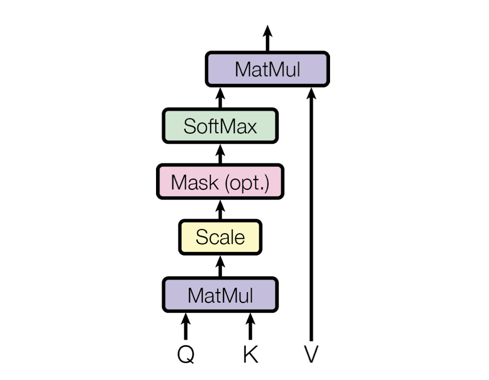
Calculating the Attention Score
The Attention Score is the dot product between every pair-wise combination of a single query and set of key vectors. It indicates how much a query should attend to a key.
💡 BIG IDEA: Recall the dot product provides us a measure of how aligned two vectors are. It is maximal when the number is large, zero when the vectors are orthogonal, and negative when they point in opposite direction. Think about what this means for a given pair of a query and key vector!
Here is an example raw attention score computation with the following inner product:
For brevity we only computed \(a_{3, 3}\) and will interpolate the rest of the value that constitute \(\vec{a}_3\) Notice the fourth attention score is what we calculated. The softmax function normalizes the dot product values into a probability distribution that sums up to one.
💡 BIG IDEA: We stabalize the raw attention score when we normalize by \(\sqrt{d_k}\) . Without it, the score would blow up the subsequent \(\text{softmax}\) to converge into a one-hot vector. In other words, the whole point of attention would be undermined, as we would only focus on one query/key pair
Again we are interpolating values for each entry of the matrix A:
W =  Q @ K.transpose(-2, -1) # (B = 1, T = 5, C = 4) @ (B = 1, C = 4, T = 5) ---> (B = 1, T = 5, T =  5)
A = F.softmax(W / K.shape[1] ** 0.5, dim=1)
O = A @ V
💡 BIG IDEA: The set of attention scores for a given query can be interpreted as a probability distribution conditioned over the keys.
Four of these attention scores are dependent on the queries assigned to all the other tokens in the sentence. So this distribution will change with each permutation of given input sentence.
These entries combined are part of a vector space representing semantic meaning.
The choice in having an attention score is probabilistic by design, presumably because there are lots of different contexts in which the word “Is” is actually used. So we want to compute the average context, conditioned on all the other words provided in the sequence.
This score is then normalized using a Softmax function (i.e. we desire having a probability).
The matrix \(\bf{O}\) represents the output of this operation, where each row is a context vector, describing the average contribution of words’ relationships to one another in a given sentence. For me this interpretation makes sense, since you are having an all-to-all relationship between key’s and queries to extract probabilistic relationships and the value represents a magnitude. So, when combined they form an average magnitude. Its a kind of sparse representation of the input sentence, now represented with machine floating points, which helps with being fed into a few feed-forward networks.
This provides us the output of one of the attention heads. Now we must concatenate multiple heads at the same time and use that larger matrix as an input into a feed-forward neural network. It has two linear transformations and a ReLU activation in between.
Feed-Forward Network
The first linear transformation is done to expand the dimensionality of the input. It represents a per-token processing. Sort of like thinking about each token, after it has processed its relationship with all the other tokens in the sequence.
For example, if the input dimension \(d_{\text{model}} = 512\) , the output dimension might be \(d_{\text{ff}} = 2048\) . In our simple of example with dimension of \(d_{\text{model}} = 4\) , we’ll expand to \(d_{\text{ff}} = 8\) , before we finally shrink back down to \(d_{\text{model}} = 4\) .
ReLU activation: This is a non-linear activation function. It’s a simple function that returns 0 if the input is negative, and the input if it’s positive. This allows the model to learn non-linear functions. The math is as follows:
$$ \text{ReLU}(x)= \max(0,x) $$
The second linear transformation reduces the dimensionality back to the original dimension. In our example, we’ll reduce from 8 to 4.
Decoder
The “Attention is All You Need” paper concerns itself with machine translation. That is converting a sequence from one language to another. For example, "Hello World, this is Alejandro! is translated into "Hola Mundo, soy Alejandro!
The Decoder utilizes Self-Attention in two places:
- Masked Self-Attention for calculating the affinity of the output generation with itself
- Encoder-Decoder Self-Attention for calculating the affinity of the output generation with the output representation of the Encoder
Masked-Multi-Head Self-Attention
💡 BIG IDEA: This self-attention layer, is for calculating the affinity of the output sequence with itself.
In other words, the Masked Attention Layer uses the self-attention computation to understand the relevance and importance of all the words that have been generated thus far and their relationship to one another.
Just as we’ve previously in the Self-Attention attention mechanism within the Encoder, the Decoder’s first sublayer applies adds positional information to embeddings, and then follows up with a masked multi-head self-attention mechanism. The embeddings however, are applied to generated data instead of an input. This matrix, representing the tokens of the already outputed generation sequence, is transformed into Q, K, and V matricies.
Where the Masked-Self Attention differs from Self-Attention, as seen in the encoder, is that we would like our attention scores to independently reflect the fact that some tokens have no awareness of what generation actually followed.
Masked Self-attention: is the mechanism that ensures the decoder only attends to the preceding words in the sequence. This means we mask the tokens that have not been generated yet.
💡 BIG IDEA: The mask is simulating an autoregressive generation process within the Decoder.
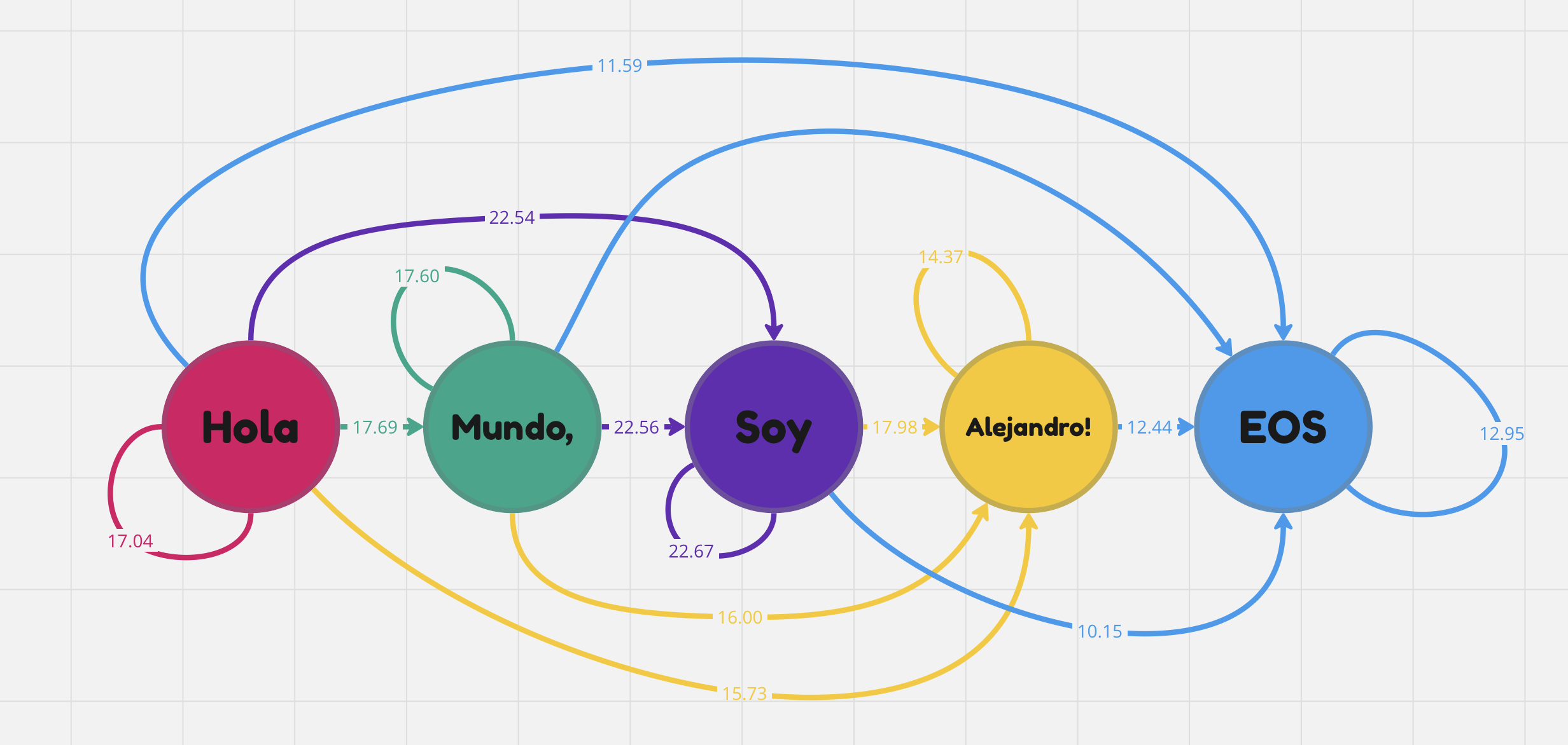
Figure X. This example generated sequence
"Hola Mundo, soy Alejandro!"illustrates how raw attention scores are derived from the relationship of each token to eachother.
We can think of attention as a communication mechanism, where each edge within a directed graph is the raw attention value between Q and V. In the figure, the token "Hola" only attends to itself with an attention of 17.04 because it represents an output generation of that word alone. However, once we get to the token "Alejandro!", we have other preceding tokens attending to the attention scores.
This is achieved by setting all the elements in the upper triangle of the scaled dot-product attention matrix (i.e., the elements that correspond to future positions) to negative infinity before applying the softmax function. Inputting negative infinity into the domain of the softmax function outputs zero. This is intentional. Here is proof.
The decoder generates future tokens one by one. This way, the mask prevents the decoder from seeing the future output tokens that have not been generated yet. The mask ensures that the attention scores for the future output tokens are very small, and thus the attention weights for them nearly zero.
Recall that for the Self-attention computation, it looked like the following:
# (B = 1, T = 5, C = 4) @ (B = 1, C = 4, T = 5) ---> (B = 1, T = 5, T =  5)
W =  Q @ K.transpose(-2, -1)

A = F.softmax(W / K.shape[1] ** 0.5, dim=1)
O = A @ V
Now, we have a matrix containing negative infinities for the top right corner we’d have something more like:
# (B = 1, T = 5, C = 4) @ (B = 1, C = 4, T = 5) ---> (B = 1, T = 5, T =  5)
W =  Q @ K.transpose(-2, -1)

# This is the Mask Matrix
M = torch.tril(torch.ones(T, T))
W = W.masked_fill(M == 0, float('-inf'))

A = F.softmax(W / K.shape[1] ** 0.5, dim=1)
O = A @ V
Encoder-Decoder Attention
Encoder-Decoder Attention (i.e. inter-attention or cross attention), the keys and values from the output derived from the full sequence of the encoder, while the queries come from the past of the sequence provided by the decoder.
Multi-Head Attention
A single self-attention mechanism is called a head, hence multi-head in the context of transformers. The same self-attention operation is done \(m\) times in parallel.
The Multi-Head Self-Attention mechanism allows the model to focus on different positions of the input sequence, capturing various aspects of the information.
This output maintains information from various representation subspaces at different positions.
Each head produces a matrix packed with context vectors, detailing the semantics of the sentence. They get concatanated together over this channel dimension. Where \(\bf{W}_O \in \mathbb{R}^{h*d_v \times d_{\text{model}}}\) . In our example, we have two heads (i.e. \(h = 2\) ), so \(\bf{W}_O \in \mathbb{R}^{10 \times 5}\) .
The authors make sure to have \(d_k = d_v = \frac{d_{\text{model}}}{h}\) .
Encoder Blocks
This part of the architecture represents a computation. You can think of it as a finite-state automata.
class Block(nn.Module):
    """ Transformer block: communication followed by computation """

    def __init__(self, n_embd, n_head):
        # n_embd: embedding dimension, n_head: the number of heads we'd like
        super().__init__()
        head_size = n_embd \\ n_head
        self.sa = MultiHeadAttention(n_head, head_size)
        self.ffwd = FeedFoward(n_embd)
        self.ln1 = nn.LayerNorm(n_embd)
        self.ln2 = nn.LayerNorm(n_embd)

    def forward(self, x):
        x = x + self.sa(self.ln1(x))
        x = x + self.ffwd(self.ln2(x))
        return x
We have stacks of these blocks processing subsequent parts of the generation.
tok_emb = self.token_embedding_table(idx) # (B,T,C)
pos_emb = self.position_embedding_table(torch.arange(T, device=device)) # (T,C)
x = tok_emb + pos_emb # (B,T,C)
x = self.blocks(x) # (B,T,C)
x = self.ln_f(x) # (B,T,C)
logits = self.lm_head(x) # (B,T,vocab_size)
Optimization Problems with Deep Neural Networks
Deep Neural Networks suffer from optimization issues. Gradient Explosion: is when small changes in the input of early layers end up being amplified in later layers. The opposite of gradient explosion is “gradient vanishing, which occurs when the gradients become too small to be useful for learning. Two common techniques to mitigate this problem are residual connections and layer normalization.
Residials
Residial Connections (i.e. Skip connections) allow the gradient to move unimpeeded throughout the computational graph, during the backwards pass in optimization. We know that the gradient-descent algorithm induces juicy statistical signals, derived from training data, into the model weights during optimization. So if we imagined gradient-descent as fire, then we might imagine residual connections as lighter fluid.
The way it works is that you have a residual pathway that works as normal. Then you have another computation that is forked off and projected back onto the residual path via addition. The reason this is useful because addition distributes gradients equally.
Each encoder (i.e. the self-attention and feedforward network) has a residual connection around it, and is followed by a layer-normalization step.
Layer Normalization
The purpose of LayerNorm is to normalize the activations during the forward pass and their gradients during the backward pass. It is implemented in PyTorch. The normalization is unit-gaussian distribution over each row in the matrix (i.e. zero mean and standard deviation of one). In the context of transformers, it is usually performed in three places:
- Applied immediately to the input prior to Multi-Head Attention Mechanism
- Applied to the output of the Multi-Head Attention Mechanism, but prior Multi-Layer Perceptron
- End of Transformer, but prior to last Linear Layer responsible for decoding tokens into the vocabulary