Driving a Data Product - Uncovering Insights and Laying out Assumptions with Exploratory Data Analysis
Table of Contents
Alejandro Armas and Sachin Loechler have been hard at work on a project that involves developing streaming workloads.
The project has the goal to process realtime data and support real-time traffic prediction! However, before I was able to begin with that. I had to demonstrate the viability of this initative. It was critical to communicate and achieve consensus on my understanding of the data with the team. In addition to learning about the data, I testing hypothesis I had and laying out the assumptions I had. What followed, was a set of requirements for a subsequent predictive system.
Why this Project Brings Value?
According to the INRIX 2022 Global Traffic Report, traffic congestion cost the US more than $81 billion in that year alone. In San Fransisco, drivers lose on average 97 hours a year due to traffic congestion. By “extra hours” they mean the extra time spent traveling at congested speeds rather than free-flow speeds.
Why Invest time into Data Analysis?
There is a large shift and amount of complexity introduced to the Machine Learning System in order to make it fully MLOPS driven.
- This complexity is usually hard to justify as time and money investments would be substantial.
Full fledged MLOps transformation is not guaranteed to bring your business a positive ROI and most certainly not in a short term. When Jeff Bezos speaks about one way door decisions and two way door decisions this project comes to mind. There is a lot of complexity to building this system, so the more upfront investment into understanding data and its limitations, the faster it is to know its not possible or the easier it is to actually plan ahead and expidite the development process.
Lessons Learned from Data
Tabular Data EDA
Performance Measurement System (PeMS) Detections
Here I started with exploratory analysis of Caltrans Performance Measurement System (PeMS). This link provided takes you to CalTrans’ clearinghouse and to download raw data in bulk, but you must create an account first.
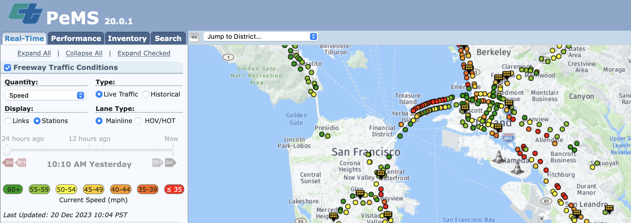
Though >39K individual detectors span the freeway system across all of the State of California, my data analysis concerned itself with 5-minute data from the North Central location in District 3. It was for I80 East, the freeway starting from San Francisco and traveling into Sacramento. The subset of data I was working with, encompassed Davis during the the two months of January in 2022 and 2023 respectively and was 3.2Gbs in size.
For those not living in the California (and especially the Bay Area), we have a pretty tame climate so I assumed there was no issue with considering only January weather, for now. Additionally, working on my local machine provided me fast signals to iterate on the analysis, but left me with limited compute. For those reasons, I reasoned the data was independently and identically distributed, and proceeded to perform data analysis on this smaller sample size.
Traffic Speed Distribution
The first step of the data analysis usually involves computing some statistics and getting a sense of how the data is distributed. Using the Plotly go.Histogram class, I was able to denote the distribution of vehicle speeds for I80 East.
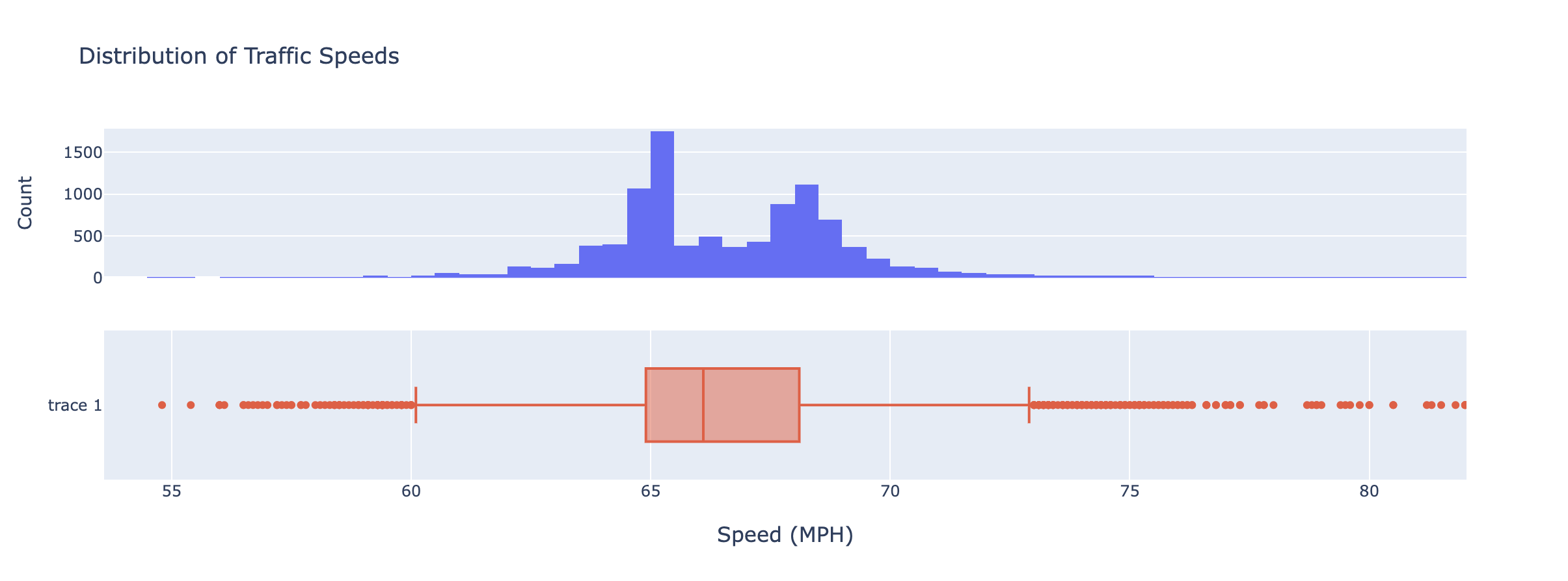
To me, it was clear that 50% of vehicles travel between 60 and 73 MPH. In these moments, it helps to draw from intuition and anecdotes. I ask myself if that makes sense. Unfortunately, I’m usually driving in the fast lane well above those speeds, so maybe not so helpful after all. Atleast I know where everyone else is at!
Traffic Speed Seasonality
The final assumption I had about the data, was that there might be some behavior in our dataset dependant on the time of the day? I wanted to observe if there existed hourly and daily seasonality.
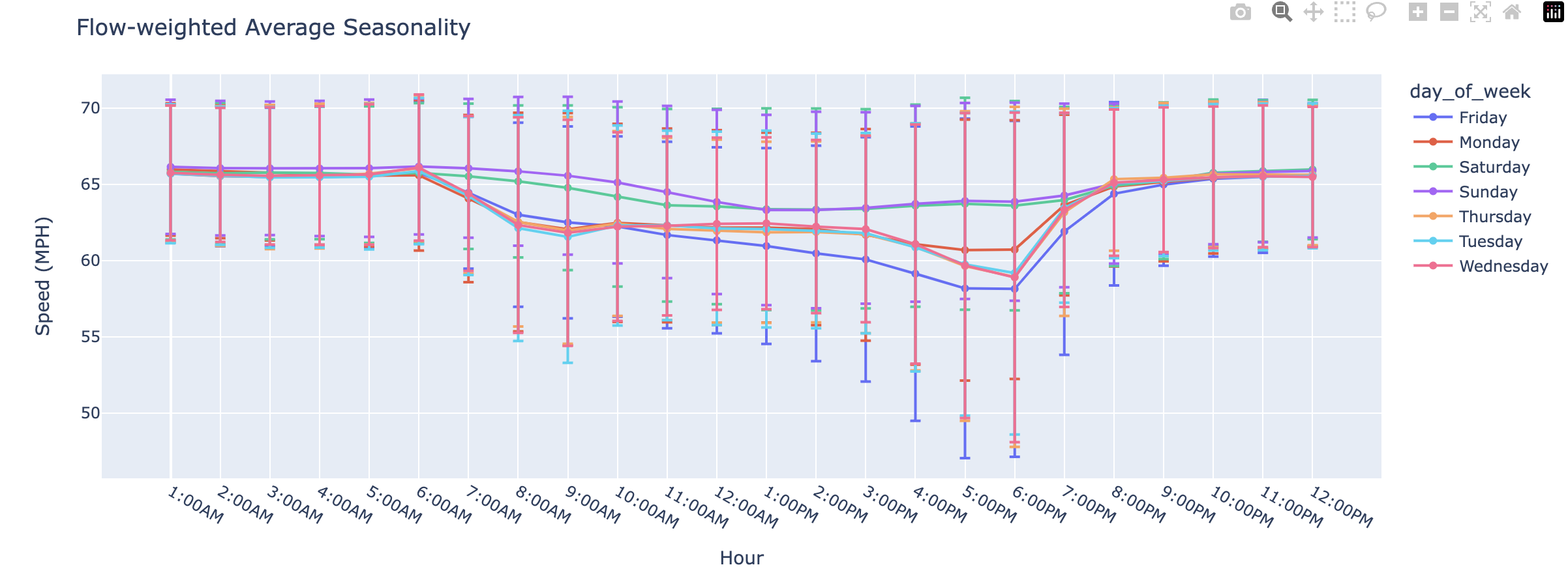
There was a clear difference between traffic speeds from weekends to weekdays. Furthermore, on weekdays traffic tended to peak from 2PM to 6PM. Anecdotely, I have observed this highway extremely congested on Fridays, which the data corroberated. Lots of Bay Area folks travel to Tahoe for the weekend. To me, this suggested that we would have to support real-time features. Specifically, time of day and weekday.
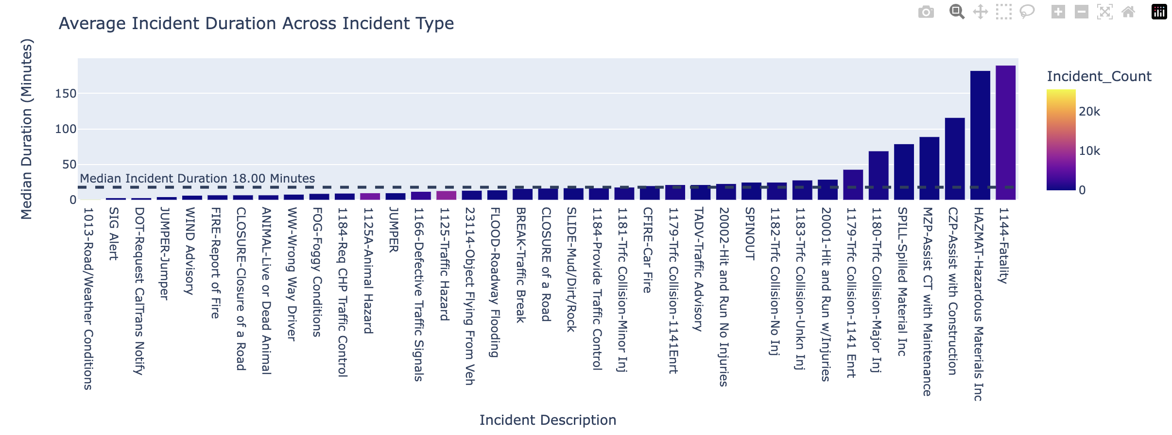
Performance Measurement System Incidents
This notebook includes exploratory analysis of Caltrans PeMS daily incident data from all california districts, during the timeframe 1/1/2022 - 1/31/2022 and 1/1/2023 - 1/31/2023 respectively.
This time-series represents incident descriptions and durations.
Traffic Incident Duration Distribution
I began by visualizing the distribution behind our incident durations. Immediately, there appears to be a decaying exponential, but most concerning of all, a lot of outliers.
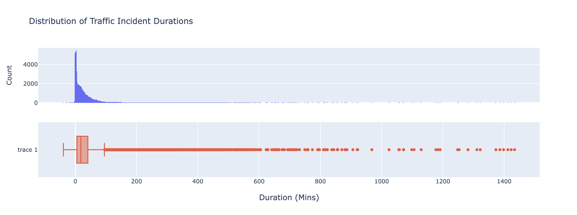
I had a couple of questions at this point. I wondered if it could be possible whether some incidents correlate with an increased delay in traffic? Likewise, I wanted to visualize how probable these longer duration incident actually were.
Working With Unstructured Video Data
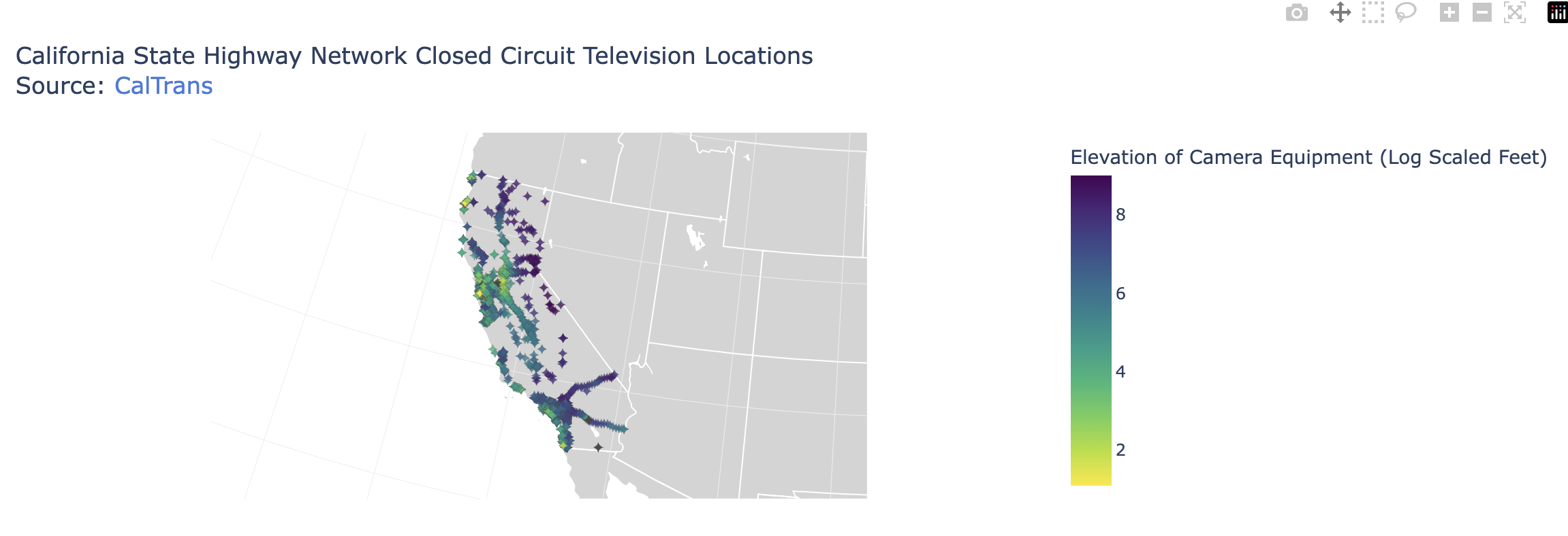
In this next section, I have graphed nodes representing PeMS traffic monitors in blue onto an interactive map via their longtitude and latitude. Additionally I overlayed livestream camera locations in red.
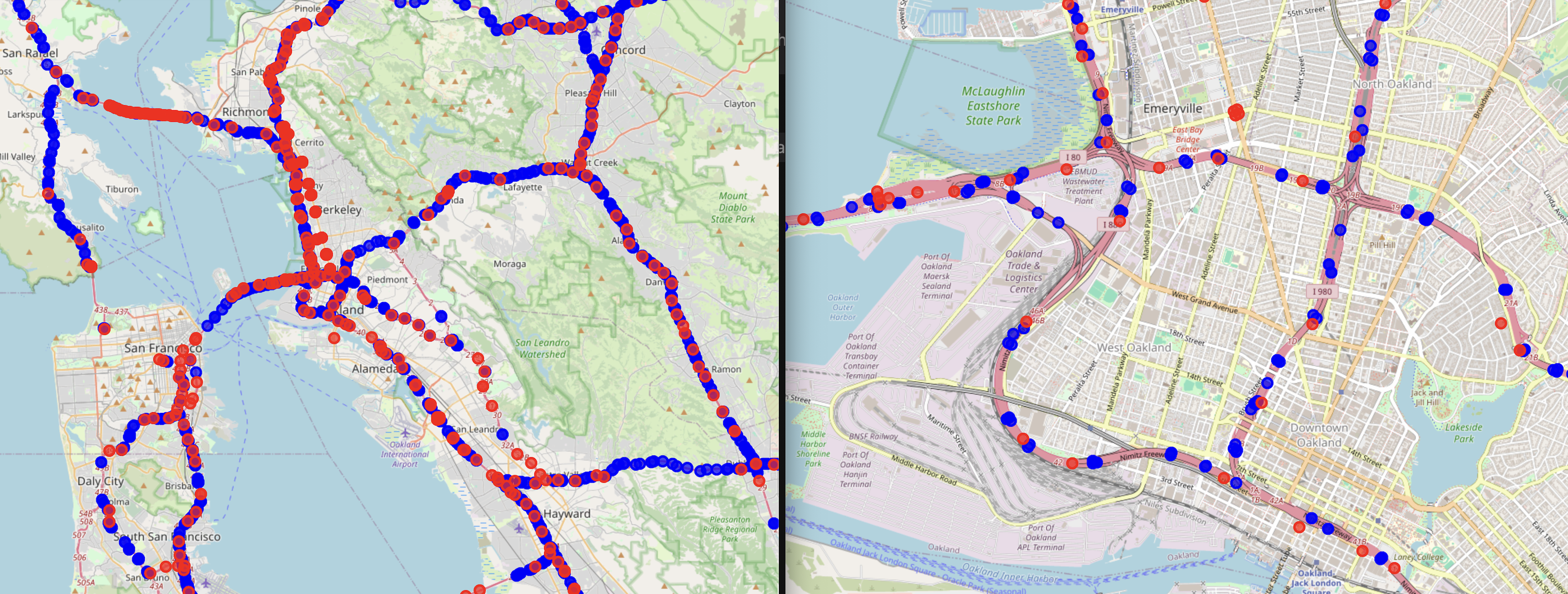
What livestream video do you ask? Lets talk about those cameras!
Caltrans provides Closed Circuit Television (CCTV) livestreams. The metadata associatiated with CCTV Caltrans footage can be found here
CCTV Metadata Exploration
This part of the analysis explores some initial requirements and feasability of a large-scale video scraper. There are a total of 2615 cameras situated across the state.
First, I wanted a sense of location for these cameras and and their status. My hypothesis was that CCTV cameras were scattered sparsely over the state. However, it turned out that they were concentrated in dense urban areas. As far as the operations go, it seemed that 46% of these livestream feeds had no link.
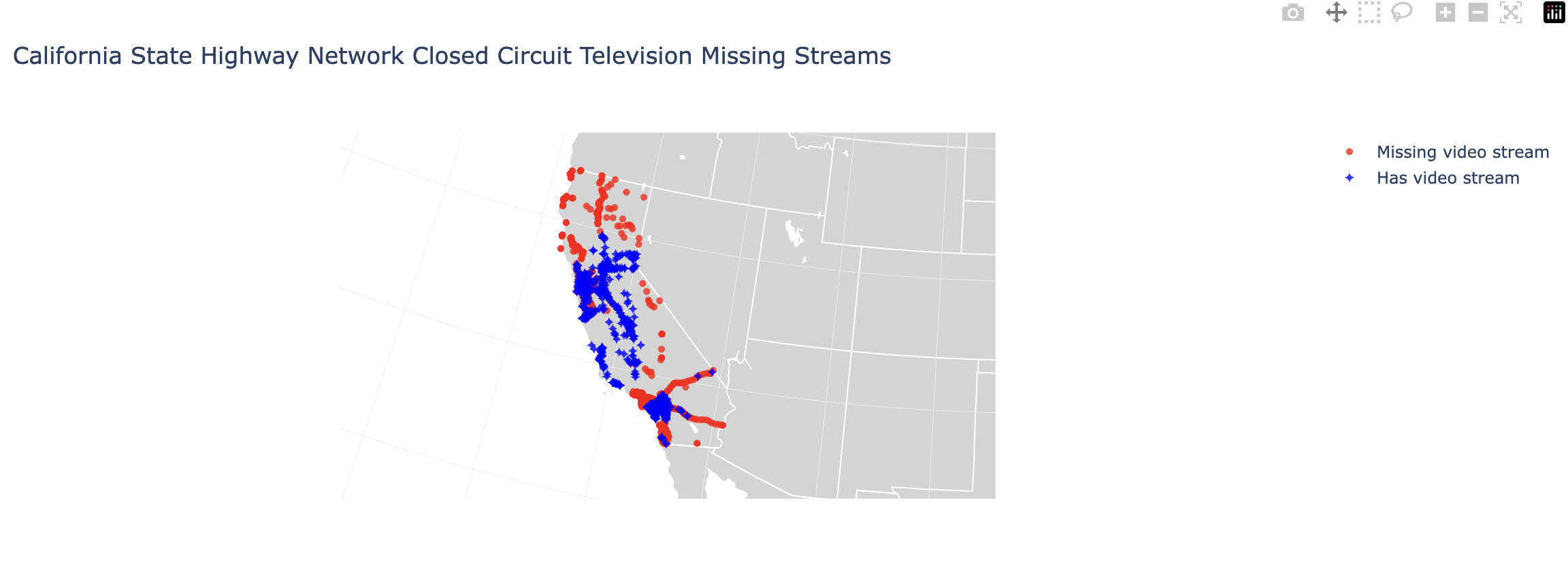
In addition to this, cameras had a field indicated if they are in service. About 54% of the cameras with a URL, actually were in service.
Next, I wanted to observe where these cameras would be in space.
Unstructured Data EDA
This section of the data analysis concerns itself with foundational models, which are pre-trained models that can learn from large-scale data and perform various downstream tasks.
They are useful for working with unstructured data, such as video footage, because they can capture the complex patterns and relationships in the data. I made use of Meta’s Cotracker + Segment Anything Model aswell as Intel’s Dense Prediction Transformer (DPT) for depth estimation and GroundingDino for bounding box creation.
CCTV Video Exploration
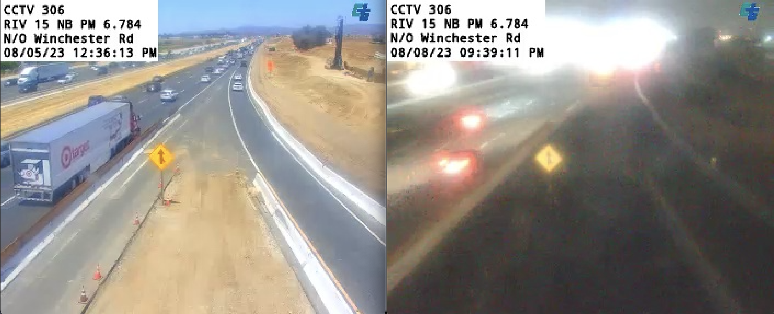
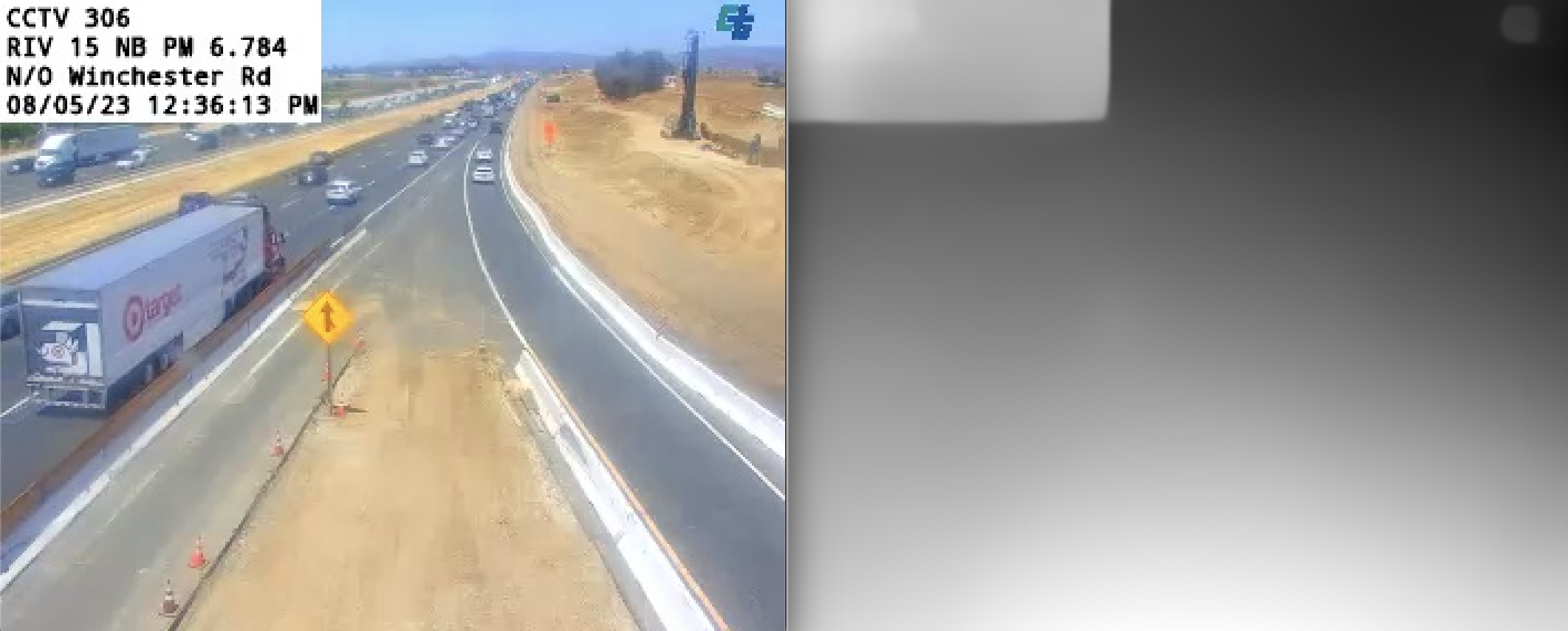
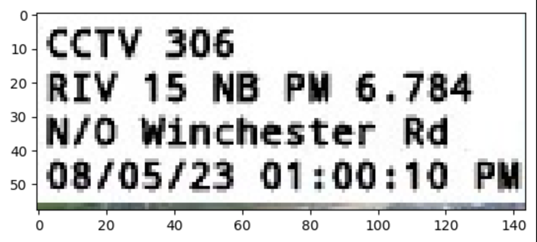
Here I feature my understanding of the (306) N/O Winchester Rd location, found in I-15 during daytime and nighttime conditions.
We include video frame analysis from livestreamed data, which we collected using:
ffmpeg -i https://wzmedia.dot.ca.gov/D8/LB-8_15_306.stream/playlist.m3u8 -t 00:30:05 -c copy -bsf:a aac_adtstoasc "LB-8_15_306.mp4"
Raw Unstructured Video Footage
Using Deep Learning, we can apply object tracking, action recognition, and scene understanding function approximators on all of this unstructured video. An important note that should be pointed out – I made sure to do analysis both in daytime and nighttime conditions. The rationale was the see the limitations of these deep learning algorithms.
Here are two frames, selected from the same freeway only days apart.
Next, we demonstrate GroundingDINO and Segment Anything Model (SAM) to be a zero-shot object detector for cars.
Bounding Boxes to Video
We wanted to filter or label data inside of our video frames, so we began with creating Bounding boxes can help locate and identify objects of interest in the video.
First, we begin with an analysis of the bounding boxes produced by GroundingDINO.
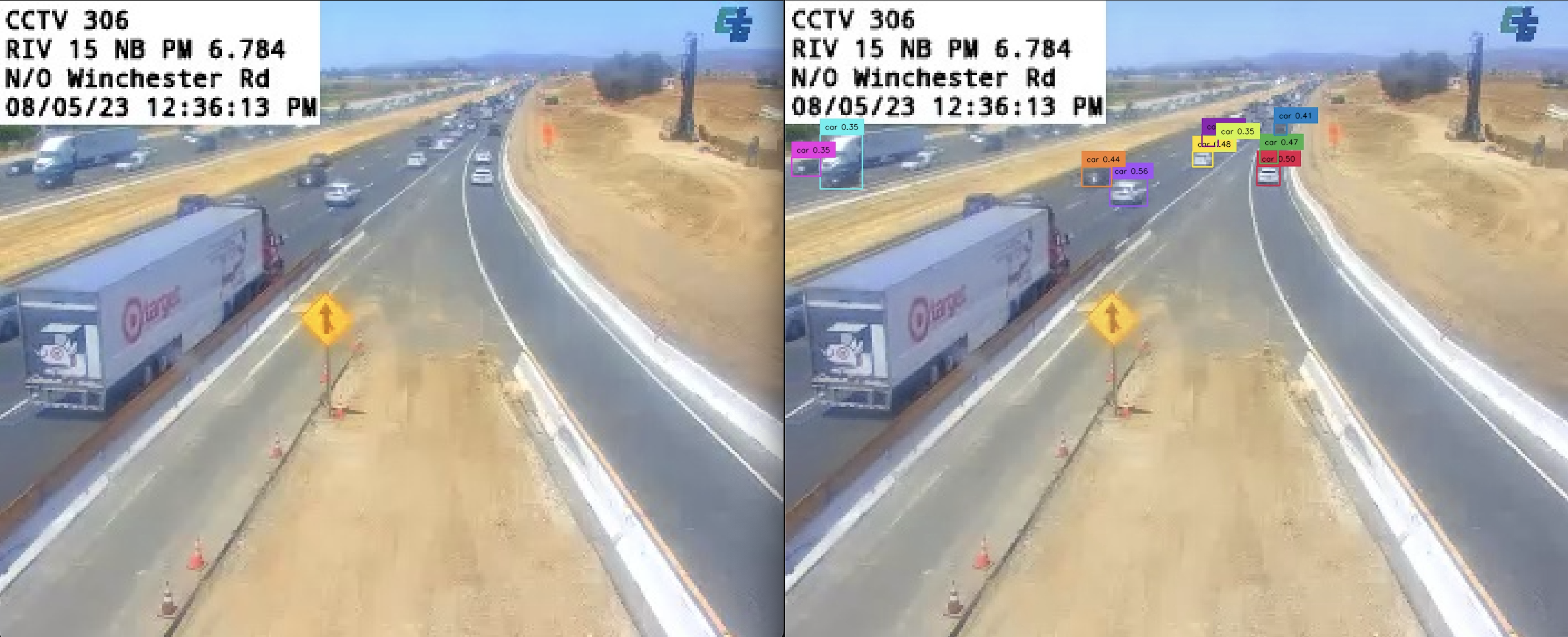
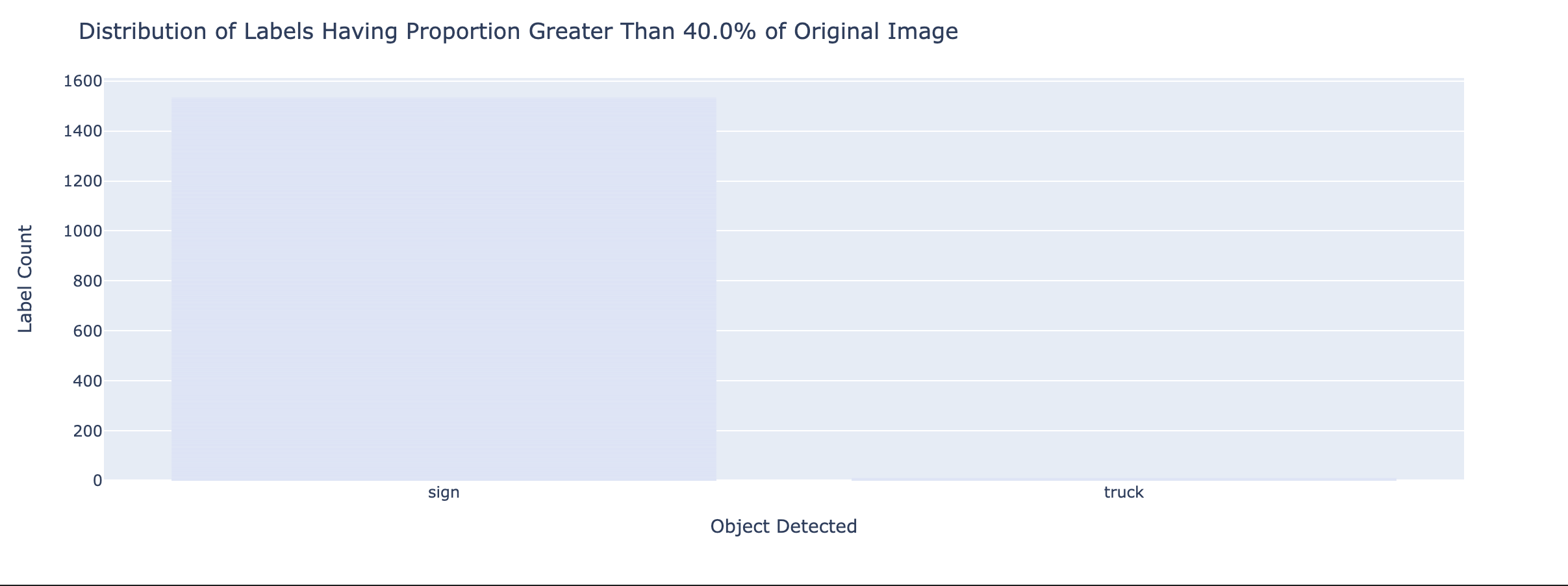
One statistic that I computed was bounding box proportion. It was a way of normalizing the length that bounding boxes occupied from their original video frame.
x_prop = df["x_width"] / image_width
You can see that on any given frame, there are generally 10 to 20 objects being detected. The legend on the right, indicates the proportion of the videoframe a bounding box takes. For instance, the objects being labeled as “sign” 1, generally takes up 40% of the video frame2. In nighttime conditions, we see that the only 1-2 objects being detected that are not “signs”.
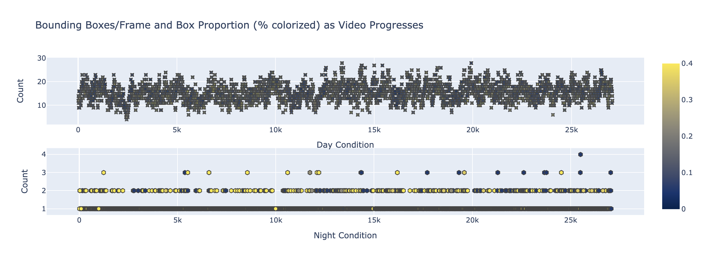
To me, this makes it very clear that without investing lots of effort into finetuning or finding better models, we will be unable to provide a service level agreement beyond hours of well illuminated video-feed.
Dense Prediction Transformer (DPT) for Monocular Depth Estimation
Here, the analysis relies on another Model, this one instead from Intel. The model estimates monocular depth perception from the CCTV’s vantage point.
Since we wanted a way of measuring or comparing features, within a frame, we thought depth perception can help estimate the distance and size of objects in the video.
Hence, we can sum all the values within of a bounding box for a given record to provide us a proxy for distance. Since some objects might take up a larger bounding box, we can simply take a mean-average.
Take note that proximity is a normalized measure. It ranges from 0 to 1. This takes hold in the next figure, where it serves as the X-axis. For the Y, we have plotted all proportions of labeled objects, conditioned by their label.
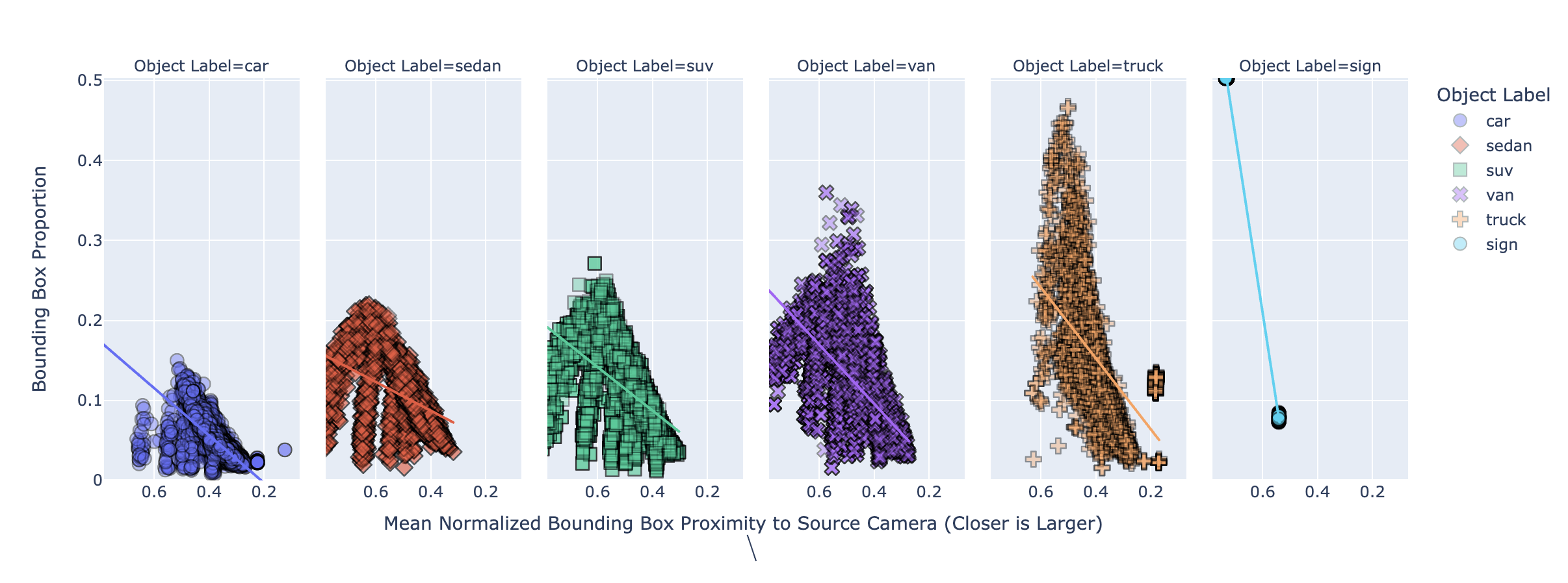
Here you can see that the Bounding Box proportions and Depth estimation measure are correlated. To me this suggests that objects are moving to or from the perspective of the video camera.
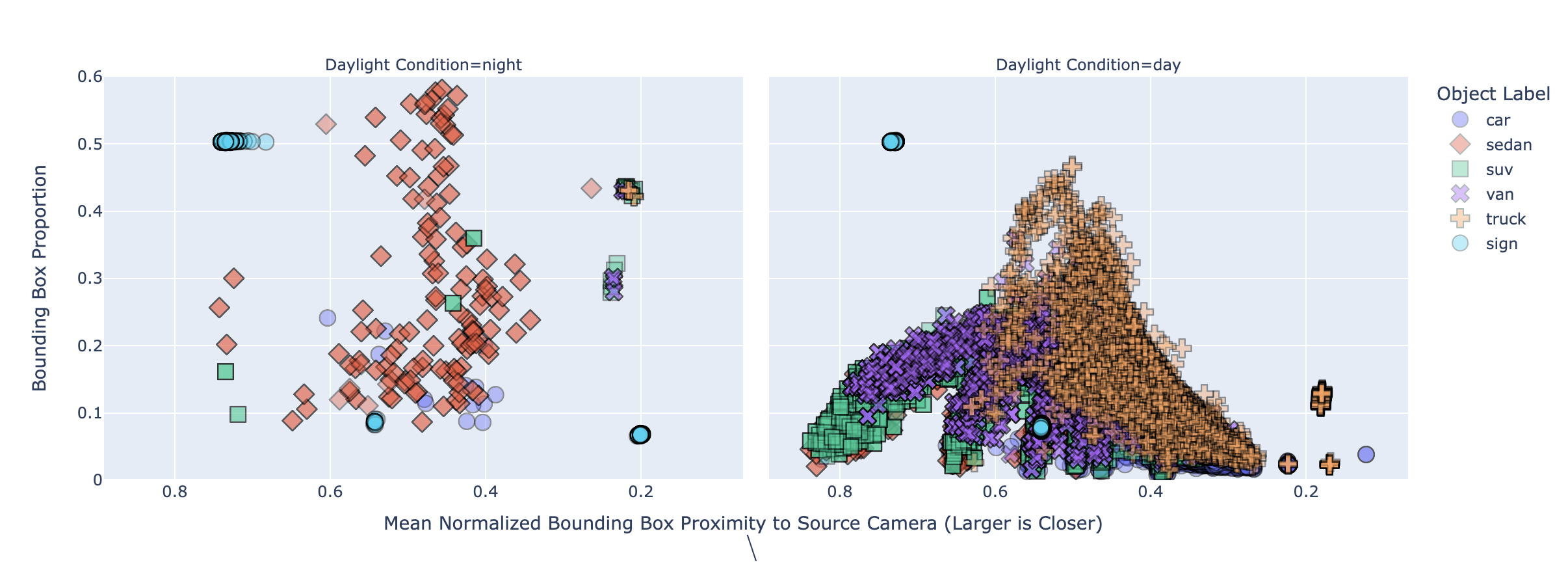
Again, we plot this data, but this time along with nighttime video footage. Needless to say, it further cements that we would not be able to provide nighttime service.
CoTracker Usage
Having lots of bounding boxes for a given frame left us with the problem with tracking the motion of objects through time. We wanted to analyze the behavior of traffic and find patterns within it, so we wanted to follow the movement and trajectory of objects in the video. I spent lots of time reasoning about algorithms to solve this until I found Co-Tracker, which does Multiple Object Tracking (MOT).
However, this presented itself with a tradeoff. A grid of points were being computed for the entire frame, so we wanted to filter this grid by points of interest. We discovered that segmentation can help separate the foreground and background of the video, which can be useful for removing noise or enhancing details of the objects labeled by the bounding boxes. We went with Segment Anything Model by Meta for this task.
Here are some of the results of my CoTracker analysis.
Predicted Tracks Lose Value as Cars go out of Frame
An example of this approach was employed, but very quickly the predicted tracks’ quality degrades once vehicles are out of the shot.
Qualitatively, it appears that for about 4 seconds, the predicted tracks follow vehicles for most frames, but quickly vanish afterwards (i.e. go out of frame). We can imagine that for faster vehicles, we would have to decrease this ceiling. Perhaps a 2s track time would be a minimum. Here is the original video footage:

Image Tracking Quality Goes Up as the Window Length Decreases
Here we employ another scenario. We are tracking objects over a 2s window. This time we apply the image segmentation pipeline onto 5 frames, spaced 2 seconds apart, and repeat for 5 smaller clips into co-tracker to obtain 5 predicted tracks, each with a duration of 2s. It looks far more accurate at the cost of performance.

Co-Tracker Performance
Co-tracker model’s weights take up about 96Mbs on disk and RAM. Using an M1 Max, it take < 15s to process 10s of a single 480x640 resolution video. This is video that has points sampled from a --grid_size 25 (i.e. 625 points filtered by the segmentation mask, resulting in 33 tracked points).
96M checkpoints/cotracker_stride_4_wind_8.pth
python demo.py --grid_size 25 --video_path assets/car-movement.mp4 --mask_pat 13.79s user 7.12s system 117% cpu 17.774 total
Grounded-Edge-SAM Performance
Using an M1 Max, it takes about 9.2 seconds to compute the bounding box and subsequent image segmentation on a 3-channel 480x640 image, for our Grounding Dino + Edge-SAM models.
python EfficientSAM/grounded_edge_sam.py 30.49s user 14.85s system 492% cpu 9.206 total
GroundingDino takes up about 662Mbs of storage and RAM for predictions, whereas Edge-SAM takes up 37Mbs.
662M Mar 20 2023 groundingdino_swint_ogc.pth
37M Dec 7 20:33 edge_sam_3x.pth
Conclusion
In conclusion, the project has the potential to reduce traffic congestion and save time for drivers by processing real-time data and supporting real-time traffic prediction. Exploratory analysis of PeMS detections and incidents provide a good starting point for further analysis and development of a predictive system. To analyze unstructured data like videos I made use of Foundational models such as Meta’s Cotracker + Segment Anything Model, Intel’s Dense Prediction Transformer (DPT), and GroundingDino for the tasks of object tracking, image segmentation, depth estimation and object labeling.
To support the viability of the realtime data prediction system, I further benchmarked the performance of these foundational models and created a list of requirements for this system.
Appendix
Labeled Sign
Labeled Sign Proportion Distribution